Saturday, December 9, 2017

PLSA using EM

PLSA using EM

Probabilistic Latent Semantic Analysis (PLSA)

We have:

  • Documents Set
  • Vocabulary Set
  • Topics

We want to find:

  • Topic Word Distribution: Word distribution the topics, for all and with the constraint .
  • Document Topic Coverage: Coverage of each topics for document , all for and with constraint .

For the rest of the note, I am skipping the background distribution for ease of mathematical notations. We define, parameter set , for . Marginal likelihood of this problem can be written as follows:


Here, since the word generation process doesn’t depend on the document, rather the topic.

E-step

Using Bayes Rule,

M-step


Using Lagrange multipler,

We get:

Summary

  • Initialize , for .

For Steps m=1, 2, … ,Do the following:

  • E-step: For and

  • M-step:

Thursday, December 7, 2017

GMM using EM

GMM using EM

Gaussian Mixture Model (GMM)

Similar to K-means clustering, however with a probabilistic flavor. That is, each point can belongs to more than one cluster, which is described by a probability distribution.

enter image description here

In the figure above, we will cluster the points using a mixture of 3 Gaussian distribution of the form , . The proportions of the Gaussian are given by . Likelihood is defined as follows:

We want to maximize the likelihood , where , . We have the following constraint:

Due to the above constraints, it is difficult to solve the problem using methods like gradient descent. So, instead, we will use EM algorithm to solve this problem.
We will convert the above likelihood function to a marginal likelihood function by introducing latent variable for . The marginal likelihood of GMM in this example as follows:

Note that, here, we have a total of probability values associated with the latent variable . However, GMM is a special case in that these mixture weights are same for all data points. So, we will only have 3 values. This is in contrast to method like PLSA, where the mixture weights are different for each data points. See here for GMM vs. PLSA. In addition, in GMM, is represented by Gaussian.

GMM: Mixture weigths are same among all data points. Also is Gaussian.

E-step

For each ,

Using Bayes Rule,

M-step


Using the assumptions specific for GMM, we can re-write the above expression as follows for 1-D input data points:

Now to determine , we set derivative to zero.

Similarly,

Solving is similar, however it also includes the constraint, and .

Summary

  • Initialize

For Steps m=1, 2, … ,Do the following:

  • E-step: For

  • M-step:


Tuesday, December 5, 2017

Expectation Maximization (EM) Algorithm

Expectation Maximization (EM) Algorithm

Reference

Objective of EM Algorithm

From wikipedia,

In statistics, an expectation–maximization (EM) algorithm is an iterative method to find ML or MAP estimates of parameters in statistical models, where the model depends on unobserved latent variables.

In the statistical model, we have:

  • - observed data
  • - unobserved latent data or missing value
  • - unknown parameters

Then:

Since, we do not observe , we need to marginalize them out.

In its general form, EM algorithm maximizes the marginal likelihood of the problem:

EM Objective

General Idea

Suppose, we want to maximize the following marginal likelihood function:

enter image description here

Similar to variational inference, here, we approximate with a family of lower bounds . Here, are known as variational parameters. In other words, we find the variational lower bounds as follows:

Initialization: Suppose, we start with point in the above figure.

enter image description here

E-step: We want to find the best lower bound from the family of lower bounds that goes through the point .

The red lower bound in the figure below is the best lower bound that goes through the point .

enter image description here

M-step: Once we found the best lower bound at E-step, as shown above, we want to find the point that maximizes the lower bound.

As shown in the figure below, is the new point.

enter image description here

Continue Iteration: As shown in the figure below.

enter image description here

E-step and KL divergence

Now, in E-step, we are trying to approximate the marginal likelihood with a family of distribution . We want to choose a distribution, that minimizes the gap shown in the figure:

enter image description here

Now, if we set Jensen’s lower bound from the above to the approximation function, i.e. , then the gap becomes:

Therefore, to minimize the gap, we will need to be zero, which will only happens when both the distributions are the same. Therefore, we have the following:

E-step
For each ,

M Step

In M-step, we want to find . Now,

Summary

In summary:
We approximate the marginal log-likelihood using a family of lower bound:

In E-step, we find best approximation of the lower bound, by maximizing over this family of lower bound, so that the gap between the marginal log-likelihood and the family of lower bound is minimized:

It turns out, the gap between marginal log-likelihood and the lower bound is equal to the KL divergence between the lower bound and
.

In M-step, we maximize the best approximation of the lower bound to find the best .

Convergence

EM algortihm converges to a local maxima.

enter image description here

In the figure above, at point , we chose the best lower bound curve during E-step. At M-step, we found where the lower bound is maximum. The likelihood at point is which is definitely higher than or equal to the lower bound at that point, i.e. .

That is the likelihood value at step k+1 is higher than the value at step k. That is, at each step, EM algorithm doesn’t lower the likelihood function. This can also be used as debugging tool.

Sunday, December 3, 2017

Bayesian Regression using PyMC3

Bayesian Regression using PyMC3

Linear regression


Here, . Therefore, we can re-write as:

In Bayesian linear regression, we assume as data and as parameters. Therefore, the likelihood is as follows:

Using Bayes rule, the posterior distribution can be written as:

Now, we can assume and to be independent of each other. We can further assume, all the elements of are independent. Therefore, prior can be written as:

Prior Distribution

  • When , then the MAP estimate is ridge regression.

  • When , i.e. Laplacian distribution, then the MAP estimate is the lasso regression.


Linear Regression using sklearn

First we import all the necessary functions:

%matplotlib inline
import numpy as np
import matplotlib.pyplot as plt
import seaborn as sns
sns.set_style("whitegrid")
sns.set_context("poster")
from sklearn.linear_model import LinearRegression
from sklearn.linear_model import Lasso, LassoCV
from sklearn.linear_model import Ridge, RidgeCV
import pymc3 as pm

We are generating some data points for the function and performing regular linear regression, Ridge regression and Lasso regression.

Ridge Regression

Lasso Regression

In our simulation, for Ridge and Lasso regression, we are intentionally setting some extreme values of so that we can see the feature selection characteristics of these regression. See this blog post for a very nice explanation of the behavior of Ridge and Lasso regression.

Note that, sklearn Ridge and Lasso doesn’t have lambda parameter, instead it has alpha parameter. My guess is, for Ridge lambda and alpha are the same. However, for Lasso, the description here is a bit confusing. After some trial and error, my suspicion is:

       alpha = number_of_samples x lambda

This is important for this analysis, since in the next section, we need to choose proper prior for our MCMC simulation depending on this value.

size = 1000 # number of data poins
np.random.seed(seed=1)

X_seed = np.random.normal(0, 1, size)
X1 = X_seed + np.random.normal(0, .1, size)
X2 = X_seed + np.random.normal(0, .1, size)
X3 = X_seed + np.random.normal(0, .1, size)

sigma = 1
noise = np.random.normal(0, sigma, size)

Y = 1 * X1 +  1 * X2 + 1 * X3 + noise

X = np.array([X1, X2, X3]).T

# Linear Regression
lr = LinearRegression()
lr.fit(X,Y)
print 'Linear model : {}'.format(lr.coef_)


# Ridge Regression (lamba = 1000)
ridge = Ridge(alpha=1000)
ridge.fit(X,Y)
print 'Ridge model : {}'.format(ridge.coef_)


# Lasso Regression
# From the description here http://scikit-learn.org/stable/modules/generated/sklearn.linear_model.Lasso.html
# I am a little confused
# my guess is lambda = alpha * n_samples
lasso = Lasso(alpha=1.)
lasso.fit(X, Y)
print 'Lasso model : {}'.format(lasso.coef_)
Linear model : [ 1.16266223  0.98860861  0.8087923 ]
Ridge model : [ 0.73644275  0.72897954  0.73591734]
Lasso model : [ 0.89910385  0.          1.02094343]

MCMC Bayesian Regression

Uniform Prior

First, we assumed uniform prior for the regression co-efficients and perform the simulation:

# using uniform prior to find the co-efficient
w_min = -10
w_max = 10

with pm.Model() as uni:
    w1 = pm.Uniform('w1', lower=w_min, upper=w_max)
    w2 = pm.Uniform('w2', lower=w_min, upper=w_max)
    w3 = pm.Uniform('w3', lower=w_min, upper=w_max)

    wTx = w1*X1 + w2*X2 + w3*X3

    y = pm.Normal('y', mu=wTx, sd=sigma, observed=Y)

    stepper=pm.Metropolis()
    traceuni = pm.sample(100000, step=stepper)
 69%|██████▉   | 69407/100500 [00:48<00:21, 1434.44it/s]

Once finished, we can plot and get summary statistics as follows:

pm.traceplot(traceuni[20000::50])
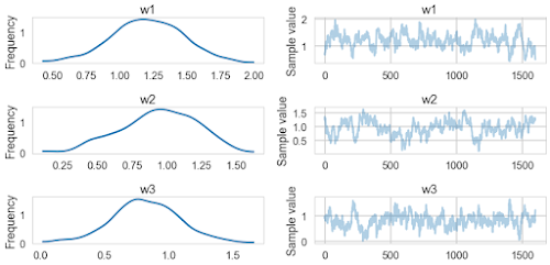
enter image description here

pm.summary(traceuni[20000::50])
w1:

  Mean             SD               MC Error         95% HPD interval
  -------------------------------------------------------------------

  1.207            0.268            0.023            [0.609, 1.688]

  Posterior quantiles:
  2.5            25             50             75             97.5
  |--------------|==============|==============|--------------|

  0.644          1.033          1.208          1.397          1.733


w2:

  Mean             SD               MC Error         95% HPD interval
  -------------------------------------------------------------------

  0.938            0.273            0.025            [0.399, 1.407]

  Posterior quantiles:
  2.5            25             50             75             97.5
  |--------------|==============|==============|--------------|

  0.400          0.764          0.952          1.147          1.408


w3:

  Mean             SD               MC Error         95% HPD interval
  -------------------------------------------------------------------

  0.819            0.262            0.022            [0.304, 1.371]

  Posterior quantiles:
  2.5            25             50             75             97.5
  |--------------|==============|==============|--------------|

  0.275          0.650          0.812          0.991          1.355

We can also try to calculate the MAP estimate of the co-efficients. This should be the same as ML estimate in the last section.

with uni:
    uni_map = pm.find_MAP()
print(uni_map)
logp = -1,447.3, ||grad|| = 4.4401: 100%|██████████| 16/16 [00:00<00:00, 1157.33it/s]  

{'w3_interval__': array(0.16224552703292178), 'w1_interval__': array(0.23723549815233705), 'w3': array(0.8094527703753798), 'w2': array(0.9728674588105903), 'w1': array(1.1806453839461994), 'w2_interval__': array(0.19519086212979697)}

Bayesian Prior - Ridge Regression

Here, we are making sure that the prior distribution of the co-efficients have zero mean and variance so that it gives us the same MAP estimate as in sklearn Ridge regression earlier.

alpha = 1000. # we used this value for sklearn Ridge estimation
lambda_1 = alpha
sigma = 1
sd = np.sqrt((sigma**2)/lambda_1)
print(sd)

with pm.Model() as ridge:
    w1 = pm.Normal('w1', mu=0, sd=sd)
    w2 = pm.Normal('w2', mu=0, sd=sd)
    w3 = pm.Normal('w3', mu=0, sd=sd)

    wTx = w1*X1 + w2*X2 + w3*X3

    ys = pm.Normal('ys', mu=wTx, sd=sigma, observed=Y)

    stepper=pm.Metropolis()
    traceridge = pm.sample(100000, step=stepper)
0.0316227766017

100%|██████████| 100500/100500 [01:11<00:00, 1402.93it/s]
pm.traceplot(traceridge[20000::50])
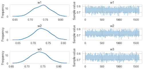
enter image description here

pm.summary(traceridge[20000::50])
w1:

  Mean             SD               MC Error         95% HPD interval
  -------------------------------------------------------------------

  0.738            0.028            0.001            [0.683, 0.789]

  Posterior quantiles:
  2.5            25             50             75             97.5
  |--------------|==============|==============|--------------|

  0.684          0.718          0.739          0.757          0.791


w2:

  Mean             SD               MC Error         95% HPD interval
  -------------------------------------------------------------------

  0.729            0.027            0.001            [0.675, 0.779]

  Posterior quantiles:
  2.5            25             50             75             97.5
  |--------------|==============|==============|--------------|

  0.676          0.711          0.729          0.748          0.783


w3:

  Mean             SD               MC Error         95% HPD interval
  -------------------------------------------------------------------

  0.738            0.027            0.001            [0.687, 0.794]

  Posterior quantiles:
  2.5            25             50             75             97.5
  |--------------|==============|==============|--------------|

  0.684          0.719          0.738          0.756          0.792

We can also estimate the MAP values for the co-efficients.

with ridge:
    mapridge = pm.find_MAP()
mapridge
{'w1': array(0.7377441385493746),
 'w2': array(0.7297896623054996),
 'w3': array(0.7369597481542057)}

Note that, these values are similar to the values obtained from sklearn Ridge.

Laplacian Prior - Lasso Regression

Note that, I am guessing the value of here due to the mismatch between the Lasso equation and sklearn implementation. The conversion in the first few line ensure that we select proper for our Laplacian priors.

alpha=1. # we used this value for sklearn Lasso
lambda_1 = alpha  * size # my guess here is, lambda = alpha x num_samples

sigma = 1.

b = sigma**2 / lambda_1
print(b)

with pm.Model() as lasso:
    w1 = pm.Laplace('w1', mu=0, b=b)
    w2 = pm.Laplace('w2', mu=0, b=b)
    w3 = pm.Laplace('w3', mu=0, b=b)

    wTx = w1*X1 + w2*X2 + w3*X3

    ys = pm.Normal('ys', mu=wTx, sd=sigma, observed=Y)

    stepper=pm.Metropolis()
    tracelaplace = pm.sample(100000, step=stepper)
0.001
100%|██████████| 100500/100500 [01:14<00:00, 1343.27it/s]
pm.traceplot(tracelaplace[20000::50])

enter image description here

pm.summary(tracelaplace[20000::50])
w1:

  Mean             SD               MC Error         95% HPD interval
  -------------------------------------------------------------------

  0.859            0.241            0.019            [0.412, 1.322]

  Posterior quantiles:
  2.5            25             50             75             97.5
  |--------------|==============|==============|--------------|

  0.389          0.695          0.863          1.034          1.304


w2:

  Mean             SD               MC Error         95% HPD interval
  -------------------------------------------------------------------

  0.179            0.141            0.009            [-0.001, 0.453]

  Posterior quantiles:
  2.5            25             50             75             97.5
  |--------------|==============|==============|--------------|

  0.007          0.068          0.145          0.255          0.551


w3:

  Mean             SD               MC Error         95% HPD interval
  -------------------------------------------------------------------

  0.890            0.237            0.020            [0.461, 1.371]

  Posterior quantiles:
  2.5            25             50             75             97.5
  |--------------|==============|==============|--------------|

  0.421          0.725          0.891          1.053          1.345

We can also find the MAP estimate:

with lasso:
    maplasso = pm.find_MAP()
maplasso
{'w1': array(0.9500293027663775),
 'w2': array(1.3861762347993195e-09),
 'w3': array(0.9796505403007957)}

Note that, this values are similar to the values estimated using sklearn Lasso earlier.

Friday, December 1, 2017

Monte Carlo Sampling

Monte Carlo Sampling

Reference


Why use Monte Carlo Sampling?

  1. To sample from a distribution - often a posterior
  2. To calculate

Here, 1 and 2 are related. If we can sample from , we can also calculate by application of law of large numbers. Suppose are i.i.d. samples drawn from . Then law of large number says:

Properties of Monte Carlo Sampling

  • Estimator is unbiased
  • Variance shrinks

Inversion Method

  • To sample from a distribution , use inverse of the CDF of the distribution and uniform random number generator.
  • CDF of a distribution is given as

    enter image description here

Steps:

  • Draw a number from uniform generator
  • Assign this number as , i.e. . Then

Cons:

  • If we can’t compute , then, we won’t be able to use this method.

Rejection Sampling Method

  • To sample from , we consider another distribution from which we can sample under the restriction - i.e., we are upper bounding the distribution with .

enter image description here

Steps:

  • Generate sample
  • Accept this sample with a certain probability. How?

    • Generate sample from a uniform distribution
    • Accept if
      Alternatively,

    • List item Generate sample from a uniform distribution

    • Accept this sample if

This method accepts points on average.

Pros:

  • Works for most distributions (even unnormalized).
  • Even works if we know our distribution up to normalization constant as it happens in probabilistic modeling, i.e. if we know , then we can upper bound by and use this method to perform sampling.

Cons:

  • In higher dimension, is high. Then, this method rejects most of the points.

Importance Sampling

Unlike Inversion method or Rejection sampling, here goal is to compute directly.

Steps:

  • Sample from a different distribution
  • Define importance weight
  • Then, is in fact

Proof:

  • In practice, we would like to choose as close as possible to to reduce the variance of our estimator

Markov Chain Monte Carlo (MCMC)

Rejection sampling and importance samplings performs poorly in higher dimensions. So, instead we use MCMC sampling.

Markov Chain

See this book for details.

  • In first order Markov chain, transition to next state depends only on previous state. A stochastic process satisfies the Markov Property if
  • For Markov chain, we have initial state and transition matrix .

enter image description here

Here,

  • Assuming the frog starts at , i.e. , then after steps, then the probability that the frog will be in or is given by

    We can also replace with a probability vector to represent the initial state - i.e. , the frog is equally likely to start in either or

Regular Markov Chain & Stationary Distribution

  • A Markov chain is regular if all the entries in the transition matrix is non-zero (this is a sufficient condition, not necessary condition).
  • For a regular Markov chain, long-range predictions are independent of the starting state, i.e. it doesn’t depend whether the frog started in or . In other words, for any choice of when . Here, is a stationary distribution such than . One interesting property is, all the entries in a column of will have the same value. E.g.

    And, for any probability vector .

A distribution is said to be invariant/ stationary w.r.t. a Markov chain if
the transition function of that chain leaves that distribution unchanged. E.g. for a Markov chain with transition operator , a distribution is considered a stationary distribution if

Detailed Balance

A transition operator satisfies detailed balance if

Here, is the stationary distribution of state , and the transition probability of moving from state to .

How to design a Markov Chain with stationary distribution

If a transition operator satisfies detailed balance w.r.t. a particular
distribution, then that distribution will be invariant under T. In other words,

Proof:

Therefore, to design a Markov Chain w.r.t. a stationary distribution , find a transition operator such that it satisfies the detailed balance w.r.t. .

How to use Markov Chain for Sampling?

  • We want to sample from
  • Build a Markov chain that converge to
    • Start from any
    • For
    • Eventually will look like samples from
      Here is the transition probability from state to .

Metropolis-Hastings Algorithm

This is somewhat similar to the idea of rejection sampling to Markov chain. We start with a wrong Markov Chain, and introduce a Critic. Critic ensures that the random walk does not go too far away from the desired distribution.

For k=1,2,
– Sample from wrong
– Accept proposal with probability
– Otherwise stay at

Transition probability of the above algorithm is as follows:

How to choose critic

We choose critic such that the transition probability as described above converged to the desired distribution . We can use detailed balance for this purpose:

Now, we assign, , then as long as . When , we can simply choose 1. I.e.

Things to note:

  • We are only using ratio of the desired distribution - this means, we don’t need to know the exact distribution. So, no issue with the normalization constant.
  • Choice of :
    • should spread out, i.e. with high variance will give us un-correlated samples. But this also means, the probability of rejection will increase. On the other had, with low variance will take long time to converge. See the following figures:

$Q$ with proper variance enter image description here enter image description here


Gibbs Sampling

We want to sample from a joint distribution

Initialize , , .
For

The 1D marginal distributions in the above algorithm can be calculated analytically or using something like rejection sampling.

Why Gibbs Sampling works?

We need to prove that the above mentioned sampling steps actually converge to stationary distribution . In other words, we need to prove:

Proof:

Metropolis-Hastings vs. Gibbs

Gibbs sampling generate highly correlated samples and takes long time to converge. Also, since sampling of each dimension depends on the past sampling from other dimension, the scheme is not parallel. Its possible to make it parallel as follows:

However, this does not guarantee that the samples will converge to the desired distribution . So, alternative is to sample from the above and use it as a proposal in Metropolis-hastings where the critic will decide whether or not to accept this point. Since, the above is pretty close the the desired distribution , there is a higher chance that the critic will accept this point.

Saturday, November 25, 2017

Notes on Bayesian Inference

Notes on Bayesian Inference

Reference

Bayes Theorem

We have,

  • : Parameters
  • : Observations

Bayes rules is as follows:

enter image description here

Probability rules:

  • Sum rules: Marginalization from joint distribution
  • Chain rules:

Point Estimation (Frequentist vs. Bayesian)

Rather than estimate the entire distribution , sometimes it is sufficient to find a single ‘good’ value for . We call this a point estimate.

  • Frequentist thinks parameters are fixed, data are random.
    Maximum Likelihood Estimation:
  • Bayesian thinks parameters are random, data are fixed.
    Maximum Aposteriori Estimation (MAP)
    • MAP estimation is not invariant to non-linear transformations of . E.g. A non-linear transformation , to can shift the posterior mode in such a way that .
    • MAP estimate may not be typical of the posterior.

Bayesian Netwok (Graphical Model)

enter image description here

  • Nodes are random variables
  • Edges indicates dependence (e.g. Grass is wet depends on both sprinkler or rain, and whether sprinkler is on or off depends on rain)
  • Observed variables are shaded nodes; unshaded nodes are hidden
  • Plated denote replicated structure

Joint probability over all the variables in the above model is given by:

enter image description here

Example 1:
enter image description here

Here,

Example 2: Naive Bayes Classifer
enter image description here

Joint Probability

In plate notation, the figure above can be shortened as follows:

enter image description here

Calculation of Posterior Distribution

  • Analytical approach: Use of conjugate prior
  • Converting to optimization problem: variational inference (mean field approximation)
  • Simulations: MCMC methods (metropolis-hastings or gibbs sampling) - see next post.

Since variational inference approximate the posterior, MCMC usually produce higher accuracy - however may be slower to converge, as shown in the figure below:

enter image description here

Conjugate Prior

Point estimation is useful for many applications, however true goal in Bayesian analysis is often to find the full posterior . In most cases, it is difficult to calculate the denominator . One approach to circumventing the integral is to use conjugate priors. Here the idea is, if we choose the ‘right’ prior for a particular likelihood function, then we can compute the posterior without worrying about the integral.

Formally, a prior is conjugate to the likelihood , if the prior and the posterior are from the same family of distribution.

Examples:

  • Beta distribution is conjugate to Bernoulli likelihood. Here is a good example of this for baseball batting average calculation.
  • Dirichlet distribution is conjugate to Multinomial likelihood (e.g. application in LDA)

Variational Inference

  • Very intuitive explanation in this blog
  • Very nice notes on the derivation from CMU here.

If there are no conjugate prior, it might be hard to calculate the posterior. In many cases, we can approximate the posterior with some known distributions.

enter image description here

Steps

We want to find posterior

  • Select a family of distribution parameterized by .
  • Find the best approximation of from by minimizing the KL divergence between the two.

Will there be issue with denominator integral?

Due to the use of KL divergence, we will have:

where . So, we don’t have to worry about .

Evidence Lower Bound (ELBO)

Evidence lower bound is defined as:

Properties: .

Proof:

Minimizing the KL divergence

We can write the KL divergence as:

Therefore,

In words, any that maximizes ELBO, minimizes KL divergence.

Mean Field Approximation

In mean field approximation, the family of distribution is assumed to factorize over the components of , i.e.

and we are trying to achieve


To get to the last line from the previous line, we did the following math:

And,

Co-ordinate Ascent

We can solve this using co-ordinate ascent algorithm, by maximizing a single factor , while keeping all other factors constant.

In summary, we first defined a family of approximations called mean field approximations, in which there are no dependencies between latent variables . Then we decomposed the ELBO into a nice form under mean field assumptions. Then, we derived a coordinate ascent updates to iteratively optimize each local variational approximation under mean field assumptions.

Common Probability Distributions

Gamma Distribution


Here,

  • support of Gamma distribution is

enter image description here

Example: Suppose I ran 5km 100 m every day, i.e. mean 5km with std 100m. We can model this as Gamma distribution. We can also use Gaussian - however, that means we can run negative distance.

enter image description here

Beta Distribution


Here,
- a, b > 0
- support of beta distribution is [0,1], i.e.
-
-

enter image description here

Example: Baseball batting average (its a number between 0 and 1). e.g.