Saturday, June 16, 2018

Logistic Regression & Metric

Logistic Regression & Metric

Logistic Regression

  • Features vector
  • We want to find the weights
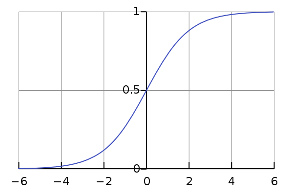
  • Classification is done using Sigmoid function:


Likelihood Approach

More compactly,

Cost/ Likelihood Function

Log-likehood function

We want to maximize the likelihood function, or minimize the negative of the likelihood function.

Graphical illustration of the cost function

  • cost = , when

  • cost = , when y=0

Solve using LMS algorithm:

Note Unlike linear regression, here, h(x) is nonlinear function of theta and x

Metric

Accuracy works well for problem when the number of positive and negative classes are not skewed. However, if one of the class is skewed, then accuracy might perform really poorly. Note that, we usually assign the class with few samples as ‘1’ and the other as ‘0’.

E.g. data set of 2000 samples with 10 positive and 1990 negative. If we assign disregarding all input , we will have accuracy of which seems quiet high - however it doesn’t learn anything.

Some other metric that we can think of is:

  • Precision/ Recall
  • F1 score
  • ROC curve
  • AUC

One way to remember this is,
TP = True Positive = Truly predicted as Positive
FN = False Negative = Falsely predicted as Negative

Precision/Recall

  • Precision: Of all the prediction predicted as positive, what percentage of them are truly positive.
  • Recall: Of all the actual positive, what percentage of them are predicted as positive.

Using the figure above:

F1 score

F1 score is a single value that combines both precision and recall. Average doesn’t work well because we wanted to give more weight to the lower of the two (precision and recall) score.

ROC Curve

Very good explanation of ROC and AUC is here. This is basically True Positive Rate vs. False Positive Rate.

AUC is the Area under the ROC curve.  

Bias-Variance Tradeoff

Bias-Variance Tradeoff

Actual model:

where is the irreducible error.

Estimation:

We approximate with

Bias and Variance of the Estimation:


Here, , since is deterministic.


MSE of estimation as a function of bias and variance of estimation


Example of bias-variance tradeoff


  • Overfitting is low bias, high variance
  • Underfitting is high bias, low variance

  • Red Line: Bias is high. Variance is low.
  • Blue Line: Bias is low. Variance is high.


Properties: Model Complexity

  • The more complex the model, the lower the bias.
  • The more complex the mode, the higher the variance.


Properties: Regularization

  • The lower the , the lower the bias, the higher the variance.
  • The higher the , the higher the bias, the lower the variance.


Properties: Number of Samples

  • Increasing sample size will decreasing variance.
  • If a learning algorithm is suffering from high bias (under-fit), getting more training data will not (by itself) help much.

  • If a learning algorithm is suffering from high variance, getting more training data is likely to help.

Summary

  • Getting more training examples fixes high variance (overfit model, use more training example)
  • Using smaller sets of features fixes high variance (overfit model, use smaller number of features)
  • Getting additional feature fixes high bias (underfit model, get more features)
  • Adding polynomial features (i.e. more complex model) fixes high variance (underfit model, increase model complexity)
  • Increasing fixes high variance (overfit model, increase )
  • Decreasing fixes high bias (underfit model, decrease )

So, for overfit model (low bias, high variance):

  • Increase sample size
  • Reduce number of features
  • Increase regularization

For underfit model (high bias, low variance):

  • Get more features
  • Increase model complexity
  • Decrease regularization

Quick Review of CNN

Quick Review of CNN

This is a summary of coursera course convolutional neural networks.

How convolution works

For horizontal edge detection, we can use:

How the edge detector works can be clear from the following figure:

Equations of Size

  • Image
  • Filter

Then:

  • Output

With Padding

If the image has a padding of on all sides, then:

  • Output

With Stride

Instead of rolling over each pixel, hop steps.

  • Output:
Padding Types
  • Valid: No padding
  • Same: Idea is to make input size and output size the same. So, use the above equation to determine the padding size that makes input and output size the same.

Convolution over Volume

  • Note Number of channels in the image must match the number of channels in the filter.
  • We sum over all dimensions at the output.

Multiple Filters

Example of CNN

  • Note each convolutional layers also contains bias term and non-linear activation (e.g. Relu).

Below is an example of a simple CNN:

Layers in a CNN

  1. Convolutional Layer: Convolution with filter (number of channels for the filter and the input must be same), Input might be padded, stride might be more than 1. Similar to a typical NN, output of the layer is the convolution layer also has bias + non-linear activation.
  2. Pooling Layer
  3. Fully Connected Layer
  4. 1X1 convolution

Pooling Layer

  • Has two hyper parameters: stride , filter size
  • Pooling layer has no parameter to learn
  • Works well in CNN - however why not well understood
  • Because nothing to learn, very cheap.

Size

Input
Hyperparameter ,
Output

Note Number of input channel and number of output channels are the same. The same filter is applied to each of the channel independently.

Example: Max Pool

Example: Average Pool

Different CNN

  • Classic
    • Lenet 5 (‘Lecun 1998)
    • AlexNet (2012)
    • VGG-16 (2015), VGG-19
  • Recent
    • ResNet (very deep 152 layers) (2015)
    • Inception (uses 1x1 convolution) (2014)

1x1 Convolution

(Network in Network, Lin et. el. 2013)
- Adds non-linearity in the network
- Help reduce number of channels if channels became too large

Example of 1x1 CONV for 1 channel image is as follows:

It seems like - it just multiplies by a constant. However, in case of multiple channel, we can think of it as a fully connected layer over the channels - i.e. , as shown in the figure below:

Example use-case to reduce number of channels:

Here, we have 32 1x1 conv filter, each of dimension 1x1x192 (192 because number of channels for input and the filter has to be the same).

LeNet

AlexNet

  • Similar to LeNet, but much bigger (60M params compare to 60K)

VGG-16

  • Simplified architecture using the same kind of operations over and over.
  • Main downside is pretty big network with ~138M params.
  • The two operations are:
    • Convolution 3x3 filters, s=1, Same
    • Pooling 2x2, s=2

ResNet

  • The issue with very deep network is the exploding/ vanishing gradient problem. ResNet makes use of ‘skip connection’ or ‘short cut’ to help with vanishing/exploding gradient problem.

Inception Net

Two key ideas:

  • Inception Block: (try out everything you want)
  • Bottleneck Layer: Reduce computational costs. E.g.

    needs 120M multiplications. In contrast, using a bottleneck layer as shown below:

    only needs 12.5M multiplications.

CART & XGBoost

CART & XGBoost

CART (Classification & Regression Trees)

CART partition the space of all joint predictor variable values into disjoint regions (see top right-hand figure). The output of the model in each of this disjoint region is a constant . That is, the predictive rule:

Output of the overall model output can be written in a more general way as follows:


Here, is the identity function, ,

At each step, CART Algorithm needs:

  • Splitting Variable
  • Splitting Point

We have observations , . If we minimize RMSE, , the best for region turns out to be the average of all the in that region :

For regression tree, to find the best variable to split on and best splitting point, we need a greedy approach. Say, we consider variable to split on at point . So, we get two region,

Then we minimize the following:

We choose the splitting point, that minimizes the above objective function. Having found the best split, we partition the data into the two resulting regions and repeat the splitting process on each of the two regions.

Boosting and Stagewise Additive Model

Boosting builds an additive models of weak learners. If is a weak learner, then we combine of such learners in a stagewise manner, i.e. at each stage , we are gonna optimize the learner , while keeping all the other learners constant. This significantly reduce the chances of overfitting.

For examples, boosting for a regression problem turns out to be the problem of repeatedly fitting the residuals, as shown below. At stage 0, the residual is the output, i.e. , . Here, is the shrinkage factor to shrink down each tree, also helps with overfitting.

For a more general framework, the forward stagewide additive model algorithm looks like this:

In boosted tree model, the weak learner is CART, and the algorithm is solved in the forward stagewise manner:

in order to find , .

At each step , the solution tree is the one that maximally reduces the above equation, given the current model and its fits .

To compare the above with a gradient descent algorithm, in gradient descent, we initialize with some random value at the first step, then in the subsequent step, we go in the negative direction of the slope.
The tree predictions here is analogous to the components of the negative gradient. The main difference is, in tree prediction, the components of the gradient vector are constrained to be the components of a decision tree, whereas in gradient descent, the negative gradient is the unconstrained maximal descent direction. In gradient boosted machine, at -th iteration, we train a tree a , whose predictions are as close as possible to the negative gradient in least-square sense:

here gradient is defined as

The following table shows gradients of the commonly use loss functions:

We can see for regression, negative gradient is just the ordinary residual .

The following algorithm shows a more generalized algorithm:

In summary, GBM involves three elements:

  1. A differentiable loss function to be optimized.
  2. A weak learner to make predictions. In this case CART
  3. An additive model to add weak learners to minimize the loss function. Trees are added one at a time, and existing trees in the model are not changed. A gradient descent procedure is used to minimize the loss when adding trees.

XGBoost

XGBoost introduced regularization and momentum term in the above formulation. Objective:

With trees, model output,

Therefore, the objective functions becomes:

Here, we can not use methods such as SGD, to find (since they are
trees, instead of just numerical vectors). So, solution is additive training:

For regression problem, we minimize the residual error at each step, as shown below:

For a more general case, we use Taylor series expansion.

Then the objective function can be approximated as:

Here,

Removing the constant, objective function becomes:

Example: Regression (again)


Then, and,

We can re-formulate tree building mechanism based on the above expansion. We can define a tree by a vector of scores in leafs , and a leaf index mapping function that maps an input instance to a leaf.

For the following tree,

Mapping function looks like:

We can define (one possible definition) the regularization term based on the above definition,

Then, for the above example, we have,

We can define the instance set in leaf as . Example, for the following input instances:

the instance set looks like: , , .
We can re-group the objective by each leaf:

This is sum of independent quadratic equations.


Using the above properties of quadratic functions, we have

Exhaustive search algorithm to find the optimum tree at step-t:

So, we can use a greedy algorithm:

Summary of XGBoost

Tree Size in each tree

Tree of size can involve variables, or interaction order of the model.